Product Lineup
From edge-based diagnostics on the factory floor to API integration into existing systems and exploratory analysis by data scientists. toorPIA technology delivered in the optimal form for your use case. Please contact us for Pricing & Licensing information.
vibeCheck
Even at low speed, the early signs show up in the sound.
Conveyors, the low-speed stage of a gearbox, agitators, cooling tower fans, rotary dryers.The slower a machine turns, the less conventional vibration diagnosis has to work with.
vibeCheck is a palm-sized diagnostic appliance with the toorPIA engine built in. Feed it the sound captured on an inspection round and it compares the recording against a base map of normal operation to find“this is not how it usually sounds”. No software rollout, no cloud subscription. It connects to neither your LAN nor the cloud, which keeps the information-security exposure small.
- No fixed sensors
- About one minute of audio from an iPhone or any recorder
- Standalone. No cloud
In service on low-speed equipment at a major chemical manufacturer
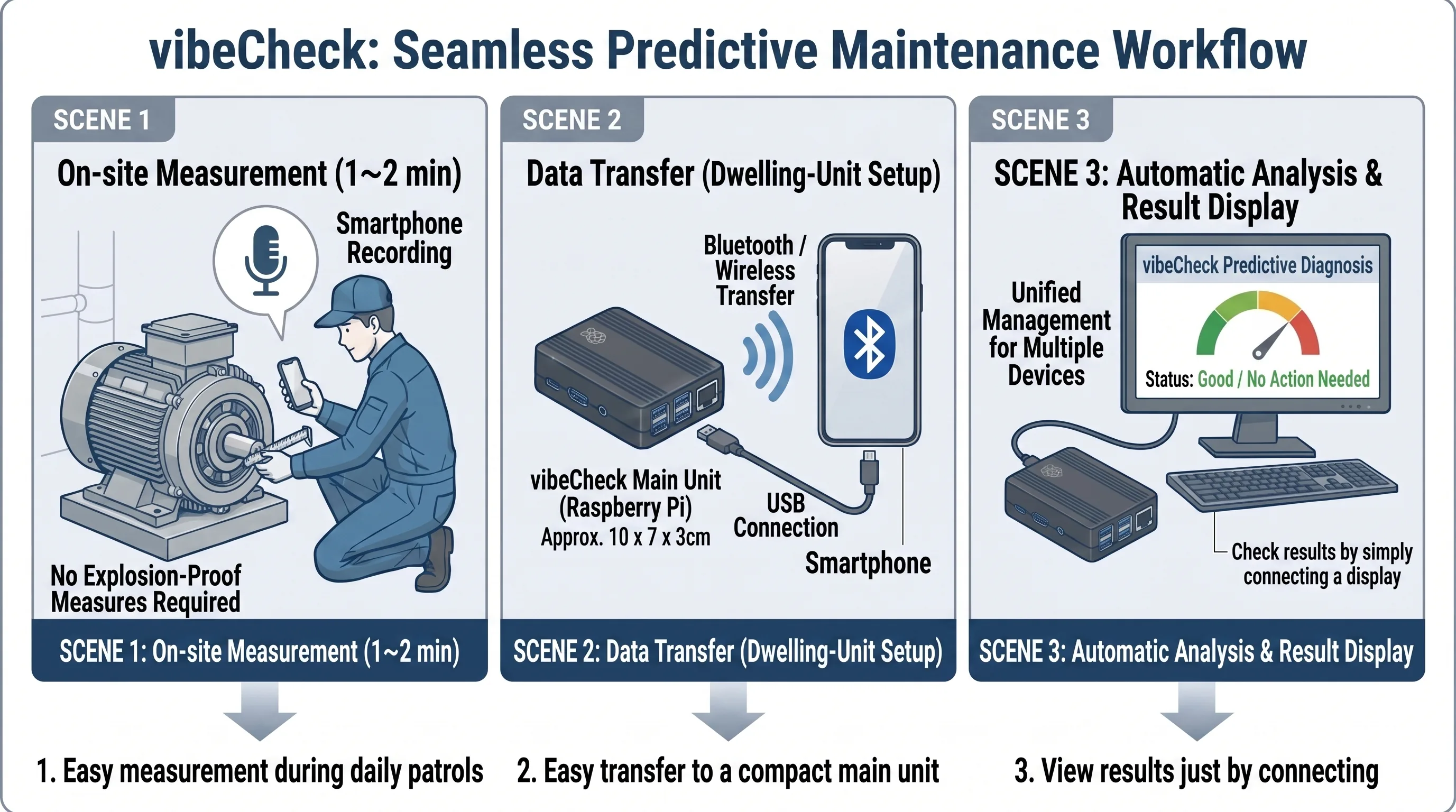
Record in the field
About one minute of audio with an iPhone or a general-purpose recorder. The recorder is the only thing you carry in. No downtime, no explosion-proofing.
Load it in the office
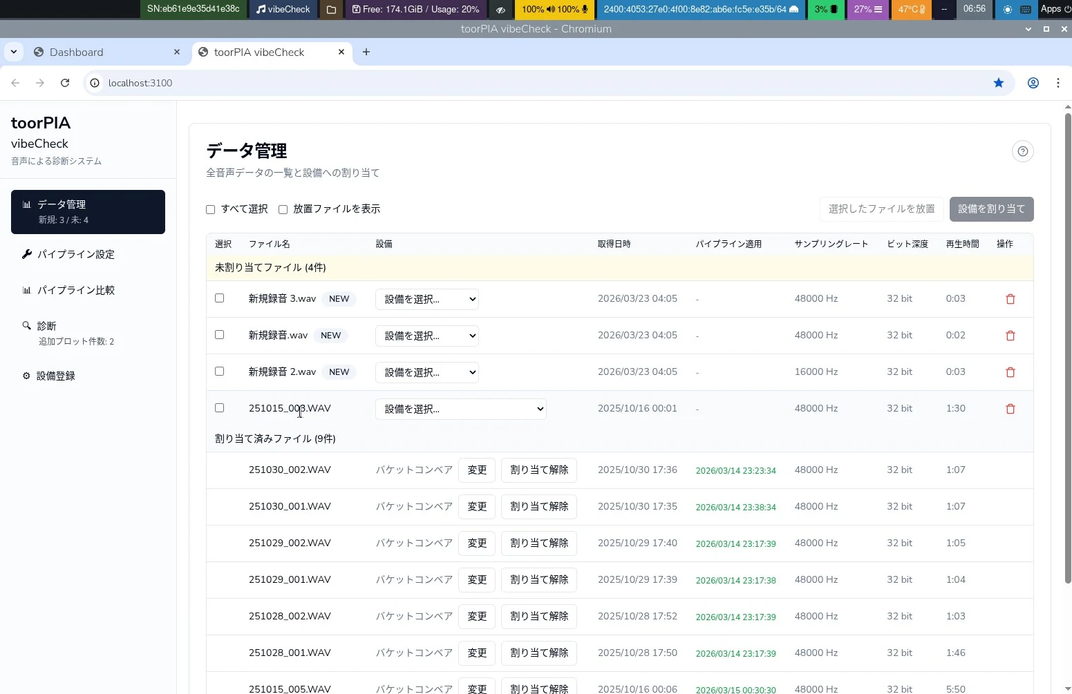
Bring the recordings to the vibeCheck unit in the office by USB, SD card or smartphone Wi-Fi. Assign them to the equipment; duplicate imports are rejected automatically.
See the result on the spot
Every import is judged automatically on a three-level scale, NORMAL / WARNING / DANGER, and a PDF report is produced.
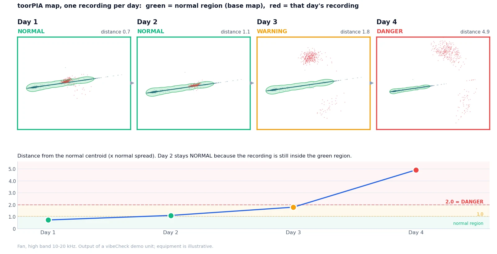
On day four, it no longer sounded normal
A fan was recorded once a day and its high band (10–20 kHz) compared against the base map. On the maps, green is the normal region and red is that day's recording. On days one and two the red points sit inside the green region: NORMAL. On day three a red cluster moves outside it: WARNING. On day four it is far away: DANGER.
The lower panel tracks the distance from the normal centroid in units of the normal spread. Day two reads 1.1 but stays NORMAL because it is still inside the green region. Nobody had to decide which frequency to watch: the day-by-day change accumulates as position and distance on the map.
Output of a vibeCheck demo unit (equipment is illustrative). How the judgment works is explained on theTechnology page, “How Precursor Monitoring Works”.
Inspection rounds become precursor diagnosis
Because you walk and record, coverage extends across the whole plant. Every round adds normal data, and a veteran's sense of “something is off” becomes a number the team can share.
- •One unit, the whole plant — Just walk with a recorder. Adding equipment is a matter of registering it
- •It matures with every round — Normal recordings accumulate and the reference map gets sharper
- •Ears become numbers — “Not the usual sound” is quantified and survives staff turnover
- •Robust to surrounding noise — Voices, hoists, carts and impacts are suppressed by the built-in preprocessing modules (10 types) so that only the machine's steady sound is judged
What it tells you, and what it does not
What you get is “this is not how it usually sounds”. It does not name the failing component. Diagnosis and the decision to act stay with your engineers — vibeCheck lets them start that work earlier. It requires data from normal operation, and recordings taken from a consistent position with a consistent technique.
Normal sound is the only reference
- •Bearing condition from audible sound — The defect may only come around a few times per second, but every impact excites the structure and shows up as sound reaching far higher frequencies. That band is where vibeCheck looks for change
- •The whole spectrum is treated as one shape — The frequency spectrum is kept as a high-dimensional vector and projected onto a 2D map by toorPIA. Nobody has to nominate which peak matters
- •Three-level judgment — Three or more normal recordings build the base map (normal region and centroid); each new recording is plotted onto it. The judgment combines inside/outside the normal region with the distance from the centroid in units of the normal spread. Guide values: NORMAL below 1.0 / WARNING 1.0–2.0 / DANGER 2.0 and above
Why low-speed machinery is hard for conventional vibration diagnosis▾
- •The signal itself is small — Excitation grows with speed. Unbalance force is proportional to the square of rotational speed, and a rolling element striking a spall hits with less force as its passing velocity drops. Meanwhile the background noise from nearby pumps and motors stays exactly where it was, so a weak signal gets buried
- •Fault repetition falls to a few events per second — Defect pass frequencies scale with shaft speed. Frequency resolution is the inverse of window length, so telling apart lines 0.1 Hz apart needs a window of 10 seconds or more. But the longer the window, the worse the time resolution — and a millisecond-long impact is averaged away (the preprocessing tradeoff)
- •Speed variation smears the peak — When load changes or a belt or chain slips, shaft speed moves and the frequency you are looking for moves with it. The more you average, the wider the peak spreads and the deeper it sinks into the floor. You can track it with a tachometer, but that means fitting one to every asset you want to watch
- •Envelope analysis needs the answer up front — Besides the band to demodulate, you need the rolling element count and dimensions, the tooth counts, and the speed of each stage before you can even compute which frequencies to look for. On multi-stage gearboxes, conveyor drivetrains and agitators, that information often simply is not on file
- •RMS velocity criteria have a lower speed bound — The evaluation zones in ISO 10816 / ISO 20816 are defined for machines down to roughly 120 r/min. Below that, the tables do not apply as written. Velocity is displacement times frequency, so the same defect reads as a smaller number the slower the machine turns
Can an anomaly be placed outside the normal region without knowing what kind of anomaly it is? We tested exactly that on a public benchmark: build the map from normal data only, then inject unseen anomaliessee the validation→
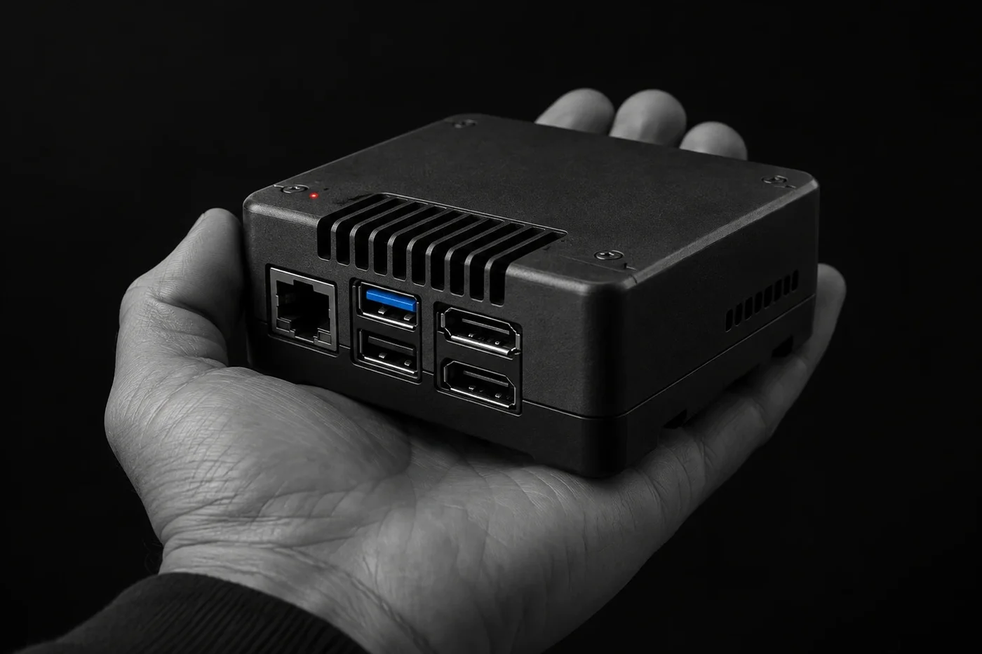
The vibeCheck unit
One box is all that arrives. Plug it in and it runs.
Unit and engine
Raspberry Pi 5 (8 GB) based, about 10 × 7 × 4 cm. toorPIA runs on the unit; no external server. NVMe SSD 500 GB (about 20,000 one-minute recordings)
Recording and input formats
iPhone microphone or a general-purpose audio recorder (piezo pickup and 32-bit float recommended). WAV (16/24/32-bit); M4A, MP3 and FLAC are converted automatically
Import and operation
Automatic import from USB and SD cards, smartphone Wi-Fi, or upload from a PC. Operate it on an HDMI monitor or a PC connected directly by LAN cable. No router, no PC settings to change
Network and support
Standalone: it does not connect to your LAN or the cloud. Remote maintenance over Soracom connectivity, with the adapter attached only when needed
Built for daily inspection
Dashboard (card color is the latest judgment), PDF reports per equipment and per round, automatic judgment and update on every import, non-destructive splitting and copying to isolate steady-state segments
Extensibility
AI-agent integration via the MCP standard. Preprocessing modules can be added as a single Python file and managed as per-equipment presets
To see how this workflow takes root on the factory floor,see our deployment approach→
toorPIA API
toorPIA's dimensionality reduction engine and precursor monitoring system delivered as a REST API. By integrating into your existing systems and data pipelines, you can monitor high-dimensional data for early warning signs that emerge in transitional regions.
From base map creation to new data projection and diagnostic score retrieval, everything is completed via API calls. Continuously monitors tens of thousands of map points in the background, with support for filtering by status and tags, and automated integration from external systems through API Key issuance.
Key Endpoints
- •Map Creation — Generate base maps from high-dimensional data. Automatic learning of normal regions
- •Data Addition & Projection — Project new data onto the base map and return 2D coordinates
- •Precursor Monitoring — Returns distance scores from the normal region and transition stages (NORMAL/WARNING/DANGER), quantifying precursory signs before anomalies develop
- •Map Management — Filtering by status and tags, dashboard integration
Technical Specifications
- •REST API / JSON format
- •Supports both batch processing and streaming
- •API Key authentication
- •Integrates with existing ETL/MLOps workflows
LLM Integration
The Python clienttoorpiaincludes a built-in MCP server, enabling LLMs such as Claude to directly perform dimensionality reduction and precursor monitoring via toorPIA.
- •Install the client and MCP server together with
pip install - •LLMs can interactively perform data analysis and precursor monitoring
For the evidence behind the engine's performance,see the open benchmark→
Create base map (submit high-dimensional data)
Project new data onto existing map
Retrieve diagnostic results
{
  "map_id": "m-2026-0401-001",
  "status": "warning",
  "score": 0.73,
  "position": { "x": 0.42, "y": -0.18 },
  "distance_from_rg": 1.84,
  "threshold_rg": 1.0,
  "in_normal_area": false
}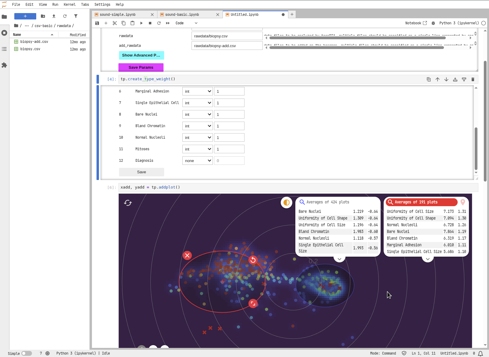
Running toorPIA in JupyterLab and performing cluster analysis with MapInspector
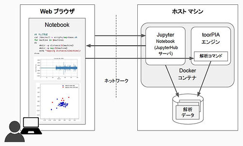
System architecture: Web Browser → JupyterHub → toorPIA Engine (inside Docker container)
toorPIA Analysis Package
An on-premises analytics platform that lets you use toorPIA in a JupyterHub + JupyterLab environment. Installed in Docker containers on your private cloud, your in-house data scientists can access the JupyterLab environment through a browser and perform exploration and analysis of high-dimensional data with toorPIA.
JupyterHub handles user authentication and session management, with each user working in an independent JupyterLab environment. The toorPIA engine is invoked as analysis commands, and results are interactively visualized within the Notebook. Data never leaves your premises, ensuring secure operations.
- •On-Premises Deployment — Secure operations without data leaving your premises. Runs in Docker containers on your private cloud
- •JupyterHub Integration — Multi-user authentication and session management. Instant access from a browser
- •MapInspector — Select clusters on projected maps and instantly compare key attribute differences. Toggle between heatmap and scatter plot views
- •Interactive Analysis — Execute commands in the Notebook to explore map creation, cluster comparison, and attribute extraction in real time
For how it tells high-dimensional states apart,see the technology page→
Pricing & Licensing
We will propose the optimal plan based on your usage scale and deployment model.
Please feel free to contact us.